Bayesian optimization with scikit-learn

Choosing the right parameters for a machine learning model is almost more of an art than a science. Kaggle competitors spend considerable time on tuning their model in the hopes of winning competitions, and proper model selection plays a huge part in that. It is remarkable then, that the industry standard algorithm for selecting hyperparameters, is something as simple as random search.

The strength of random search lies in its simplicity. Given a learner \(\mathcal{M}\), with parameters \(\mathbf{x}\) and a loss function \(f\), random search tries to find \(\mathbf{x}\) such that \(f\) is maximized, or minimized, by evaluating \(f\) for randomly sampled values of \(\mathbf{x}\). This is an embarrassingly parallel algorithm: to parallelize it, we simply start a grid search on each machine separately.

This algorithm works well enough, if we can get samples from \(f\) cheaply. However, when you are training sophisticated models on large data sets, it can sometimes take on the order of hours, or maybe even days, to get a single sample from \(f\). In those cases, can we do any better than random search? It seems that we should be able to use past samples of \(f\), to determine for which values of \(\mathbf{x}\) we are going to sample \(f\) next.

Bayesian optimization

There is actually a whole field dedicated to this problem, and in this blog post I’ll discuss a Bayesian algorithm for this problem. I’ll go through some of the fundamentals, whilst keeping it light on the maths, and try to build up some intuition around this framework. Finally, we’ll apply this algorithm on a real classification problem using the popular Python machine learning toolkit scikit-learn. If you’re not interested in the theory behind the algorithm, you can skip straight to the code, and example, by clicking here.

Bayesian optimization¹ falls in a class of optimization algorithms called sequential model-based optimization (SMBO) algorithms. These algorithms use previous observations of the loss \(f\), to determine the next (optimal) point to sample \(f\) for. The algorithm can roughly be outlined as follows.

1. Using previously evaluated points \(\mathbf{x}_{1:n}\), compute a posterior expectation of what the loss \(f\) looks like.
2. Sample the loss \(f\) at a new point \(\mathbf{x}_{\text{new}}\), that maximizes some utility of the expectation of \(f\). The utility specifies which regions of the domain of \(f\) are optimal to sample from.

These steps are repeated until some convergence criterion is met.

Gaussian processes as a prior for functions

To compute a posterior expectation, we need a likelihood model for the samples from \(f\), and a prior probability model on \(f\). In Bayesian search, we assume a normal likelihood with noise

in other words, we assume \(y \vert f \sim \mathcal{N}(f(\textbf{x}), \sigma^2_\epsilon)\).

For the prior distribution, we assume that the loss function \(f\) can be described by a Gaussian process (GP). A GP is the generalization of a Gaussian distribution to a distribution over functions, instead of random variables. Just as a Gaussian distribution is completely specified by its mean and variance, a GP is completely specified by its mean function \(m(\textbf{x})\), and covariance function \(k(\textbf{x}, \textbf{x}')\).

For a set of data points \(\textbf{x}_{1:n} = \{\mathbf{x}_1, \ldots, \mathbf{x}_n\}\), we assume that the values of the loss function \(f_{1:n} = \{f(\mathbf{x}_1), \ldots, f(\mathbf{x}_n)\}\) can be described by a multivariate Gaussian distribution

where \(m(\mathbf{x}_{1:n}) = \left[m(\mathbf{x}_1), \ldots, m(\mathbf{x}_n) \right]^T\), and the \(n \times n\) kernel matrix \(\textbf{K}\) has entries given by

We can think of a GP as a function that, instead of returning a scalar \(f(\textbf{x})\), returns the mean and variance of a normal distribution over the possible values of \(f\) at \(\textbf{x}\).

A GP is a popular probability model, because it induces a posterior distribution over the loss function that is analytically tractable. This allows us to update our beliefs of what \(f\) looks like, after we have computed the loss for a new set of hyperparameters.

Acquisition functions

To find the best point to sample \(f\) next from, we will choose the point that maximizes an acquisition function. This is a function of the posterior distribution over \(f\), that describes the utility for all values of the hyperparameters. The values with the highest utility, will be the values for which we compute the loss next.

What does an acquisition function look like? There are multiple proposed acquisition functions in the literature, but the expected improvement (EI) function seems to be a popular one. It is defined as

where \(\hat{\textbf{x}}\) is the current optimal set of hyperparameters. Maximising this quantity will give us the point that, in expectation, improves upon \(f\) the most.

The nice thing about the expected improvement is, that we can actually compute this expectation under the GP model, by using integration by parts.

where \(\Phi(z)\), and \(\phi(z)\), are the cumulative distribution and probability density function of the (multivariate) standard normal distribution.

This closed form solution gives us some insight into what sort of values will result in a higher expected improvement. From the above, we can derive that;

1. EI is high when the (posterior) expected value of the loss \(\mu(\textbf{x})\) is higher than the current best value \(f(\hat{\textbf{x}})\); or
2. EI is high when the uncertainty \(\sigma(\textbf{x})\) around the point \(\textbf{x}\) is high.

Intuitively, this makes sense. If we maximize the expected improvement, we will either sample from points for which we expect a higher value of \(f\), or points in a region of \(f\) we haven’t explored yet (\(\sigma(\textbf{x})\) is high). In other words, it trades off exploitation versus exploration.

Putting all the pieces together

After all this hard work, we are finally able to combine all the pieces together, and formulate the Bayesian optimization algorithm:

1. Given observed values \(f(\textbf{x})\), update the posterior expectation of \(f\) using the GP model.
2. Find \(\textbf{x}_{\text{new}}\) that maximises the EI: \(\textbf{x}_{\text{new}} = \arg \max EI(\textbf{x}).\)
3. Compute the value of \(f\) for the point \(\textbf{x}_{\text{new}}\).

This procedure is either repeated for a pre-specified number of iterations, or until convergence.

When looking at the second step, you may notice that we still have to maximize another function, the acquisition function! The nice thing here, is that the acquisition function is a lot easier to optimize than the original loss \(f\). In case of the EI acquisition, we can even compute the derivatives analytically, and use a gradient-based solver to maximise the function.

Finally, we can get to some coding! Because scikit-learn has a Gaussian process module, we can implement this algorithm on top of the scikit-learn package. In pseudocode, the Bayesian optimization algorithm looks as follows:

import sklearn.gaussian_process as gp

def bayesian_optimization(n_iters, sample_loss, xp, yp):
  """

  Arguments:
  ----------
    n_iters: int.
      Number of iterations to run the algorithm for.
    sample_loss: function.
      Loss function that takes an array of parameters.
    xp: array-like, shape = [n_samples, n_params].
      Array of previously evaluated hyperparameters.
    yp: array-like, shape = [n_samples, 1].
      Array of values of `sample_loss` for the hyperparameters
      in `xp`.
  """

  # Define the GP
  kernel = gp.kernels.Matern()
  model = gp.GaussianProcessRegressor(kernel=kernel,
                                      alpha=1e-4,
                                      n_restarts_optimizer=10,
                                      normalize_y=True)
  for i in range(n_iters):
    # Update our belief of the loss function
    model.fit(xp, yp)

    # sample_next_hyperparameter is a method that computes the arg
    # max of the acquisition function
    next_sample = sample_next_hyperparameter(model, yp)

    # Evaluate the loss for the new hyperparameters
    next_loss = sample_loss(next_sample)

    # Update xp and yp

A proper Python implementation of this algorithm can be found on my GitHub page here.

Parameter selection of a support vector machine

To see how this algorithm behaves, we’ll use it on a classification task. Luckily for us, scikit-learn provides helper functions, like make_classification(), to build dummy data sets that can be used to test classifiers.

from sklearn.datasets import make_classification

data, target = make_classification(n_samples=2500,
                                   n_features=45,
                                   n_informative=15,
                                   n_redundant=5)

We’ll optimize the penalization parameter \(C\), and kernel parameter \(\gamma\), of a support vector machine, with RBF kernel. The loss function we will use, is the cross-validated area under the curve (AUC), based on three folds.

from sklearn.model_selection import cross_val_score
from sklearn.svm import SVC

def sample_loss(params):
  C = params[0]
  gamma = params[1]

  # Sample C and gamma on the log-uniform scale
  model = SVC(C=10 ** C, gamma=10 ** gamma, random_state=12345)

  # Sample parameters on a log scale
  return cross_val_score(model=model,
                         X=data,
                         y=target,
                         scoring='roc_auc',
                         cv=3).mean()

Because this is a relatively simple problem, we can actually compute the loss surface as a function of \(C\) and \(\gamma\). This way, we can get an accurate estimate of where the true optimum of the loss surface is.

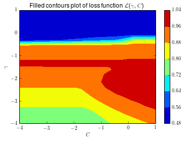
For the underlying GP, we’ll assume a Matern kernel as the covariance function. Although we skim over the selection of the kernel here, in general the behaviour of the algorithm is dependent on the choice of the kernel. Using a Matern kernel, with the default parameters, means we implicitly assume the loss \(f\) is at least once differentiable. There are a number of kernels available in scikit-learn, and each kernel implies a different assumption on the behaviour of the loss \(f\).

The animation below shows the sequence of points selected, if we run the Bayesian optimization algorithm in this setting. We also warm-start the procedure with 5 random samples from \(f\). The star shows the value of \(C\) and \(\gamma\) that result in the largest value of cross-validated AUC.

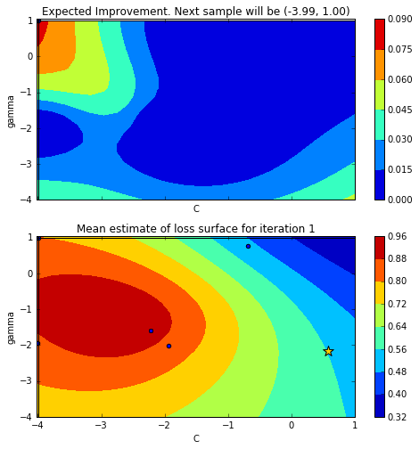
This is quite cool! Initially, the algorithm explores the parameter space a bit, but it quickly discovers a region where we have good performance, and it samples points in that region. This definitely is a smarter strategy than random search!

Tips and tricks

Unfortunately, it is not always that easy to get such good results with Bayesian optimisation. When I was just looking into this method, I was hoping for a simple algorithm, in which I could just plug in my data and model, and wait for the optimal solution to come out (like the grid search methods in scikit-learn).

However, to tune your original machine learning model with this algorithm, it turns out you have to put considerable effort into tuning the search algorithm itself! I have found that the following are some practical things to consider:

1. Choose an appropriate scale for your hyperparameters: For parameters like a learning rate, or regularization term, it makes more sense to sample on the log-uniform domain, instead of the uniform domain.

2. Kernel of the GP: Different kernels have a drastic effect on the performance of the search algorithm. Each kernel implicitly assumes different properties on the loss \(f\), in terms of differentiability and periodicity.

3. Uniqueness of sampled hyperparameters: Sampled hyperparameters that are close to each other, reduce the condinitioning of the problem. A solution is to add jitter (noise) to the diagonal of the covariance matrix. This is equivalent to adding some noise through the alpha parameter of the GaussianProcessRegressor method. Make sure that the order of magnitude of the noise is on the appropriate scale for your loss function.

Wrapping up

Bayesian optimisation certainly seems like an interesting approach, but it does require a bit more work than random grid search. The algorithm discussed here is not the only one in its class. A great overview of different hyperparameter optimization algorithms is given in this paper².

If you’re interested in more production-ready systems, it is worthwhile to check out MOE, Spearmint³, or hyperopt⁴. These implementations can also deal with integer, and categorical, hyperparameters.

An interesting application of these methods are fully automated machine learning pipelines. By treating the type of model you want to estimate as a categorical variable, you can build an optimizer in the hyperopt framework, that will select both the right model type, and the right hyperparameters of that model (see section 2.2 here, for an example). It seems that this makes a large part of my job as a data scientist obsolete, but luckily we are not completely there yet!

References