Filtering the noise with stability selection

In the previous blog post, I discussed different types of feature selection methods and I focussed on mutual information based methods. I’ve since done a broader talk on feature selection at PyData London. In the talk, I discussed an example of an embedded feature selection method called stability selection, a method that tends to work well in high-dimensional, sparse, problems.

Embedded methods are a catch-all group of techniques that perform feature selection as part of the model construction process. They typically take the interaction between feature subset search and the learning algorithm into account, at the cost of extra computational time.

Structure learning

Stability selection¹ wraps around an existing structure learning algorithm, and tries to enhance and improve it. The goal of these kind of algorithms is to learn the underlying relationships of the data. Structure learning can take different forms, but one example is the LASSO algorithm for supervised regression. Here, the algorithm tries to determine which features relate to the target variable, and the (covariance) structure is then defined as the set of features with non-zero values for their coefficients in the final linear model.

Other examples of such structure learning algorithms are:

• Orthogonal Matching Pursuit (number of steps in forward selection)
• Matching Pursuit (number of iterations)
• Boosting (L1 penalty)

What these structure learning algorithms typically have in common is a parameter \(\lambda \in \Lambda\) that controls the amount of regularisation, mentioned above within the parentheses. For every value of \(\lambda\), we can obtain a structure estimate \(\hat{S}^{\lambda} \subseteq \{1, \ldots, p\}\), that indicates which features to select. Here, \(p\) is the total number of available features, the dimensionality of our problem.

Enhancing the structure learning algorithm

The rough idea behind stability selection is to inject more noise into the original problem by generating bootstrap samples of the data, and to use a base structure learning algorithm to find out which features are important in every sampled version of the data.

For a feature to be considered stable (or important), it has to be selected in a high number of perturbed versions of the original problem. This tends to filter out features that are only weakly related to the target variables, because the additional noise introduced by the bootstrapping breaks that weak relationship.

To make the above more precise, we have to dive into the mathematical details. The algorithm takes as input a grid of regularization parameters \(\Lambda\), and the number of subsamples \(N\) that need to be generated. Stability selection returns a selection probability \(\hat{\Pi}^\lambda_k\) for every value \(\lambda \in \Lambda\) and for every feature \(k\), and the set of stable features \(\hat{S}^{\text{stable}} \subseteq \{1, \ldots, p\}\).

The algorithm consists of two steps. In the sampling step the selection probabilities, or stability scores, are computed as follows. For each value \(\lambda \in \Lambda\) do:

• For each \(i\) in \(1, \ldots, N\), do:

  • Generate a bootstrap sample of the original data \(X^{n \times p}\) of size \(\frac{n}{2}\).
  • Run the selection algorithm on the bootstrap sample with regularization parameter \(\lambda\) to get the selection set \(\hat{S}_i^\lambda\).

• Given the selection sets from each subsample, calculate the empirical selection probability for each model component:

In the scoring step we then compute the set of stable features according to the following definition

where \(\pi_\text{thr}\) is a predefined threshold. The algorithm is also represented in the following diagram

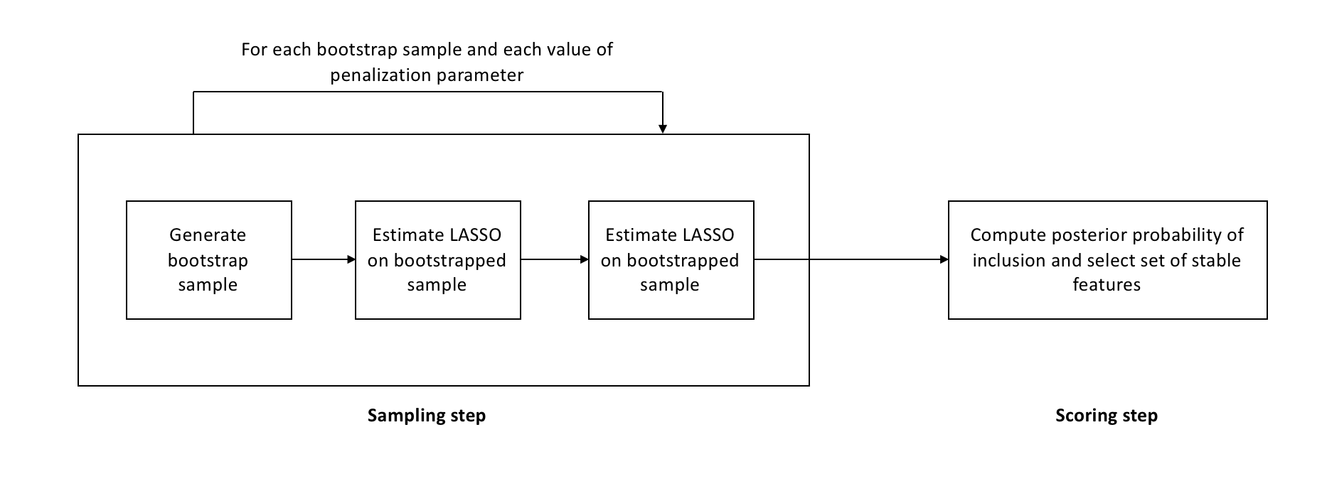
The base algorithm is run on every bootstrap sample for a grid of values of the penalization parameter, and not just a single value. A-priori we don’t know what the right level of regularization for a problem is. If a variable is related to the target variable in a meaningful way, it should show up in most bootstrap samples for at least one value of the penalization parameter.

When the stability score for a variable exceeds the threshold \(\pi_\text{thr}\) for one value in \(\Lambda\), it is deemed stable. This means that some regularization is necessary. In specific cases one can obtain minimum bounds (as obtained in the Meinshausen and Buhlmann paper), but in general this requires some fiddling around with the mathematical details.

Implementing it in Python

Stability selection is actually relatively straightforward to implement. If you have an implementation of the base learner available, the algorithm can wrap around that and it is only necessary to write the bootstrapping and scoring code. Both of these two steps don’t require sophisticated mathematics. Roughly speaking, an implementation could look as follows:

import numpy as np


def stability_selection(lasso, alphas, n_bootstrap_iterations,
                        X, y, seed):
  n_samples, n_variables = X.shape
  n_alphas = alphas.shape[0]

  rnd = np.random.RandomState(seed)
  selected_variables = np.zeros((n_variables,
                                 n_bootstrap_iterations))
  stability_scores = np.zeros((n_variables, n_alphas))

  for idx, alpha, in enumerate(alphas):
    # This is the sampling step, where bootstrap samples are generated
    # and the structure learner is fitted
    for iteration in range(n_bootstrap_iterations):
      bootstrap = rnd.choice(np.arange(n_samples),
                             size=n_samples // 2,
                             replace=False)

      X_train = X[bootstrap, :]
      y_train = y[bootstrap]

      # Assume scikit-learn implementation
      lasso.set_params({'C': alpha}).fit(X_train, y_train)
      selected_variables[:, iteration] = (np.abs(lasso.coef_) > 1e-4)

    # This is the scoring step, where the final stability
    # scores are computed
    stability_scores[:, idx] = selected_variables.mean(axis=1)

  return stability_scores

I’ve put a Python implementation of stability selection with a scikit-learn compatible API on my GitHub. Since stability selection is model-agnostic, you can plug in any scikit-learn estimator that has a coef_ or feature_importances_ attribute after fitting:

base_estimator = Pipeline([
    ('scaler', StandardScaler()),
    ('model', LogisticRegression(penalty='l1'))
])

selector = StabilitySelection(base_estimator=base_estimator, lambda_name='model__C',
                              lambda_grid=np.logspace(-5, -1, 50)).fit(X, y)

print(selector.get_support(indices=True))

A useful diagnostic for stability selection is plotting the stability path. This is similar to plotting the LASSO path, and it is a plot of the stability scores versus the values of the penalization parameter, plotted for every variable.

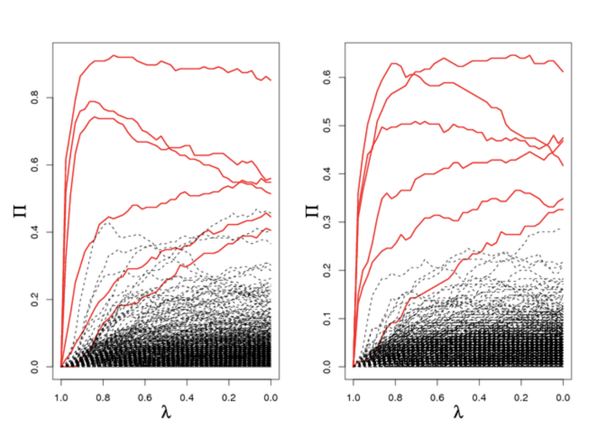
The above figure is taken from the original stability selection paper¹. It can be used to understand how stable the scores are, and can also help distinguish which variables are more important, within the set of selected variables.

Bells and whistles

Note that there are some bells and whistles that can be added to an implementation of stability selection:

• The bootstrapping parts are easily parallelizable, and in certain cases (LASSO regression) one can use efficient implementations of the base algorithm to get results even faster (lasso path).
• Different sampling schemes can also be used for stability selection. For example, a complementary pairs bootstrapping procedure, where one data point is never in two consecutive bootstrap samples, is discussed in ².

Stability selection has proven highly effective in some of the problems I have dealt with. In this post I have skipped over some details, but the papers cited contain more motivations and theoretical guarantees behind the algorithm. The original paper¹ is also interesting because they propose to inject even more noise into the problem, by using a learner called the randomised LASSO that essentially takes a random value \(\lambda \in \Lambda\). The details in this post should give you enough to start using this method in your work, but do read the references for the interesting stuff!

References