Long-term forecasting with machine learning models

Time series analysis has been around for ages. Even though it sometimes does not receive the attention it deserves in the current data science and big data hype, it is one of those problems almost every data scientist will encounter at some point in their career. Time series problems can actually be quite hard to solve, as you deal with a relatively small sample size most of the time. This usually means an increase in the uncertainty of your parameter estimates or model predictions.

A common problem in time series analysis is to make a forecast for the time series at hand. An extensive theory around on the different types of models you can use for calculating a forecast of your time series is already available in the literature. Seasonal ARIMA models and state-space models are quite standard methods for these kinds of problems. I recently had to provide some forecasts and in this blog post I’ll discuss some of the different approaches I considered.

The difference with my previous encounters with time series analyses was that now I had to provide longer term forecasts (which in itself is an ambiguous term, as it depends on the context) for a large number of time series (~500K). This prevented me from using some of the classical methods mentioned before, because

1. classical ARIMA models are typically well-suited for short-term forecasts, but not for longer term forecasts due to the convergence of the autoregressive part of the model to the mean of the time series; and
2. the MCMC sampling algorithms for some of the Bayesian state-space models can be computationally heavy. Since I needed forecasts for a lot of time series quickly this ruled out these type of algorithms.

Instead, I opted for a more algorithmic point of view, as opposed to a statistical one, and decided to try out some machine learning methods. However, most of these methods are designed for independent and identically distributed (IID) data, so it is interesting to see how we can apply these models to non-IID time series data.

Forecasting strategies

Throughout this post we will make the following non-linear autoregressive representation (NAR) assumption. Let \(y_t\) denote the value of the time series at time point \(t\), then we assume that

for some autoregressive order \(n\) and where \(\epsilon_t\) represents some noise at time \(t\) and \(f\) is an arbitrary and unknown function. The goal is to learn this function \(f\) from the data and obtain forecasts for \(t + h\), where \(h \in \{1, \ldots, H\}\). Hence, we are interested in predicting the next \(H\) data points, not just the \(H\)-th data point, given the history of the time series.

When \(H = 1\) (one-step ahead forecasting), it is straightforward to apply most machine learning methods on your data. In the case where we want to predict multiple time periods ahead (\(H > 1\)) things become a little more interesting.

In this case there are three common ways of forecasting:

• iterated one-step ahead forecasting;
• direct \(H\)-step ahead forecasting; and
• multiple input multiple output models.

Iterated forecasting

In iterated forecasting, we optimize a model based on a one-step ahead criterion. When calculating a \(H\)-step ahead forecast, we iteratively feed the forecasts of the model back in as input for the next prediction. In Python, a function that computes the iterated forecast might look like this:

def generate_features(x, forecast, window):
    """ Concatenates a time series vector x with forecasts from
        the iterated forecasting strategy.

    Arguments:
    ----------
        x:        Numpy array of length T containing the time series.
        forecast: Scalar containing forecast for time T + 1.
        window:   Autoregressive order of the time series model.
    """
    augmented_time_series = np.hstack((x, forecast))

    return augmented_time_series[-window:].reshape(1, -1)

def iterative_forecast(model, x, window, H):
    """ Implements iterative forecasting strategy

    Arguments:
    ----------
        model: scikit-learn model that implements a predict() method
               and is trained on some data x.
        x:     Numpy array containing the time series.
        h:     number of time periods needed for the h-step ahead
               forecast
    """
    forecast = np.zeros(H)    
    forecast[0] = model.predict(x.reshape(1, -1))

    for h in range(1, H):
        features = generate_features(x, forecast[:h], window)

        forecast[h] = model.predict(features)

    return forecast

To understand the disadvantage of this method a bit better, it helps to go back to the original goal of our problem. What we are really trying to do is to approximate

where

and

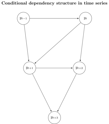
where \(n\) is the order of the autoregressive model. We can visualize this distribution using a graphical model. In the case \(n = 2\), the distribution of the time series data can be represented as follows

We don’t actually know the real values of \(y_{t + 1}, y_{t + 2}\) and \(y_{t + 3}\). Instead, we use our forecasts \(\hat{y}_{t + 1}, \hat{y}_{t + 2}\) and \(\hat{y}_{t + 3}\). As a result, the distribution of our approximation looks like this

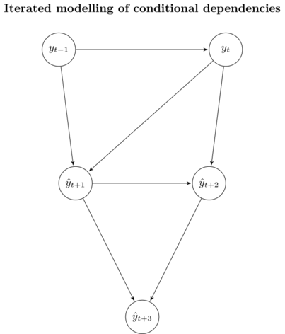
The iterated strategy returns an unbiased estimator of \(\mathbb{E}\left[ \textbf{y}_{(t+1):(t+H)} \,\vert\, \textbf{y}_{(t-n+1):t} \right]\), since it preserves the stochastic dependencies of the underlying data. In terms of the bias-variance trade-off, however, this strategy suffers from high variance due to the accumulation of error in the individual forecasts. This means that we will get a low performance over longer time horizons \(H\).

Direct \(H\)-step ahead forecasting

In direct \(H\)-step ahead forecasting, we learn \(H\) different models of the form

where \(h \in \{1, \dots, H\}\), \(n\) is the autoregressive order of the model, and \(f_h\) is any arbitrary learner. Training the models \(f_h\) in Python is relatively straightforward, as you only need to use different (lagged) versions of your training data and response.

def ts_to_training(x, window, h):
    """ Generates a training and test set from a time series
        assuming we want to calculate a h-step ahead forecast.

    Arguments:
    ----------
        x: Numpy array that contains the time series.
        h: Number of periods to forecast into the future.
    """
    n = x.shape[0]
    nobs = n - h - window + 1

    features = np.zeros((nobs, window))
    response = np.zeros((nobs, 1))

    for t in range(nobs):
        features[t, :] = x[t:(t + window)]
        response[t, :] = x[t + window]

    return features, response


def direct_forecast(model, x, window, H):
    """ Implements direct forecasting strategy

    Arguments:
    ----------
        model: scikit-learn model that implements fit(X, y) and
               predict(X)
        x:     history of the time series
        H:     number of time periods needed for the H-step ahead
               forecast
    """
    forecast = np.zeros(H)

    for h in range(1, H + 1):
        X, y = ts_to_training(x, window=window, h=h)

        fitted_model = model.fit(X, y)

        forecast[h - 1] = fitted_model.predict(X[-1, :].reshape(1, -1))

    return forecast

The distribution this strategy approximates can again be visualized in a graphical model:

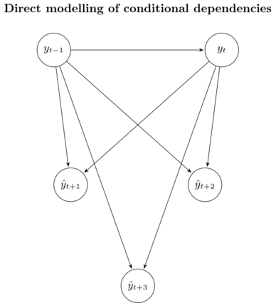
Here, we see that this approach does not suffer from the accumulation of error, since each model \(f_h\) is tailored to predict horizon \(h\). However, since the models are trained independently, no statistical dependencies between the predicted values \(y_{t + h}\) are guaranteed.

An alternative strategy, called the DirRec strategy¹, can be used to mitigate this problem. The idea is to still train \(H\) different models, but we use the forecasts of the earlier periods more and more as we predict further into the future. Even though this deals with the conditional independence assumption, the strategy is computationally heavy because we now need to train \(H\) independent models.

Multiple input multiple output (MIMO) models

Finally, we can also train one model that takes multiple inputs and returns multiple outputs:

The forecasts are provided in one step, and any learner \(f\) that can deal with a multi-dimensional response can be used (yes, you can go crazy with your 12-layer neural network). We only need to transform the time series \(y_t\) such that you can feed it into the learner \(f\). In Python, this could look like this.

def ts_to_mimo(x, window, h):
    """ Transforms time series to a format that is suitable for
        multi-input multi-output regression models.

    Arguments:
    ----------
        x:      Numpy array that contains the time series.
        window: Number of observations of the time series that
                will form one sample for the multi-input multi-output
                model.
        h:      Number of periods to forecast into the future.
    """
    n = x.shape[0]
    nobs = n - h - window + 1

    features = np.zeros((nobs, window))
    response = np.zeros((nobs, h))

    for t in range(nobs):
        features[t, :] = x[t:(t + window)]
        response[t, :] = x[(t + window):(t + window + h)]

    return features, response

The results of the above function can then be piped into any model that takes multi-dimensional input and output data. In long term prediction scenarios, both the iterated (because of the accumulation of errors in the forecasts) and direct strategies neglect stochastic dependencies between future values. The main advantages of the MIMO forecasting strategy are that

1. only one model is trained instead of \(H\) different models;
2. no conditional independence assumptions are made (c.f. direct strategy); and
3. there is no accumulation of error of individual forecasts (c.f. iterated strategy).

Using models that take multi-dimensional inputs and outputs therefore seems like the most natural choice of models for forecasting.

One constraint of the MIMO strategy is that all horizons \(H\) are to be forecasted with the same model, which limits our flexibility. One approach to combat this assumption is to combine the direct and MIMO strategy, and is called the DIRMO strategy². The general idea is to split the forecasting horizon \(H\) into \(m = \frac{H}{b}\) blocks of length \(b\) (where \(b \in \{1, \ldots, H\}\)). We then train \(m\) different models, where each model is used to predict one of the blocks in a MIMO fashion.

Final words

Out of the three strategies discussed here the MIMO strategy seems to be the most natural approach to applying machine learning methods to long-term forecasting problems.

However, when it comes to forecasting there is no silver bullet and what works best may be problem specific. One downside of using machine learning methods for forecasting problems (or any non-parametric model for that matter) is that we can’t quantify the uncertainty in our predictions in terms of frequentist confidence or Bayesian credible intervals. This problem can perhaps be partly mitigated by using the block bootstrap to get bootstrapped confidence intervals.

If your ultimate goal is more explanatory rather than predictive in nature, you may find that more classical models like state-space models will give you better bang for your buck. Bayesian dynamic linear models (DLMs) in particular work nicely here, because of their flexibility and ease of interpretation (check out this post over at Stitch Fix for an excellent discussion of these models).

References